Notes about GCN Sampling

I read several papers about Sampling Algorithm in Graph Convolution Network training last week. So I wrote this note to simply record them.

METHOD	SAMPLING SCHEME	CONFERENCE
GraphSAGE	node-wise	NIPS 17
FastGCN	layer-wise	ICLR 18
StochasticGCN	node-wise	ICML 18
AdaptiveSampling	layer-wise	NIPS 18
ClusterGCN	?node-wise	KDD 19

GraphSAGE

Paper Link

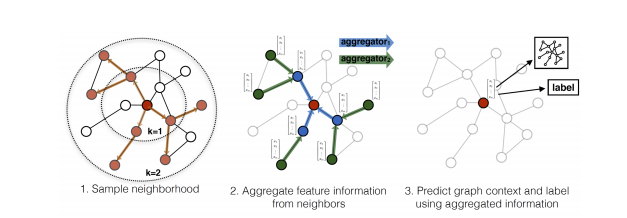
This sampling method is uniform sampling and very easy to understand. It uses a Top-down approach, which means that when it is calculating a node’s output, the algorithm finds the node’s neighbors layer by layer, until the node’s representation vector can be calculated.

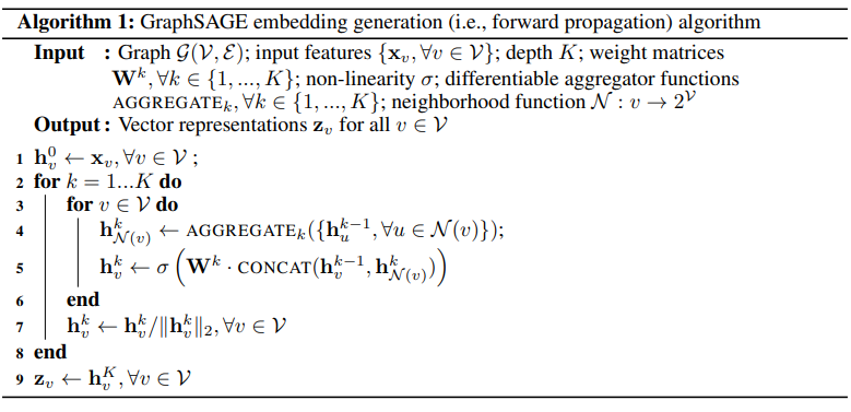
In my opinion, this paper was not made for Sampling. It just use a simple and naive uniform sampling trick to avoid too heavy calculation. The main purpose of this paper might just be to make the train of GCN can be processed in a batch manner.

FastGCN

Paper Link

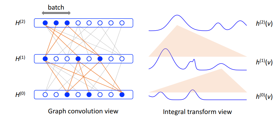
This paper rewrites the Message Passing formula in am integral form, then uses Monte Carlo Sampling to approximate the integral value.

$$
\tilde{h}{t+1}(v)=\int \hat{A}(v, u) h^{(l)}(u) W^{(l)} d P(u), h^{(l+1)}(v)=\sigma\left(\tilde{h}^{(l+1)}(v)\right), \quad l=0, \ldots, M-1 $$
$$
L=\mathrm{E}{v \sim P}\left[g\left(h^{(M)}(v)\right)\right]=\int g\left(h^{(M)}(v)\right) d P(v) $$
$$
\tilde{h}{t{l+1}}^{(l+1)}(v) :=\frac{1}{t_{l}} \sum_{j=1}^{t_{l}} \hat{A}\left(v, u_{j}^{(l)}\right) h_{t_{l}}^{(l)}\left(u_{j}^{(l)}\right) W^{(l)}, h_{t_{l+1}}^{(l+1)}(v) :=\sigma\left(\tilde{h}{t{l+1}}^{(l+1)}(v)\right), \quad l=0, \ldots, M-1
$$

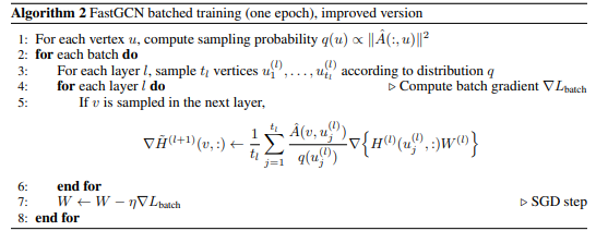
It uses a factor proportional to the degree of the node as the importance sampling factor.

StochasticGCN

Paper Link

The algorithm is not complicated in this paper, but this paper provides many theoretical results and proofs.

The algorithm is that when aggregating neighbors’ features/activations, only a few of neighbors will actually computes their activations, while the others will use the historical activations as approximation.

It can be easily derived that in the end when the message passing reaches a stationary point, the sampling variance will be eliminated to zero.

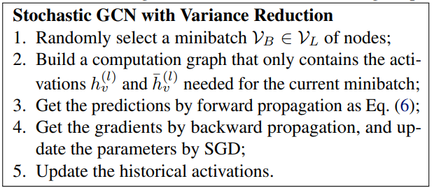
Along with the insight, the paper also provides the convergence guarantee and variance analysis. It has high theoretical value.

Adaptive Sampling

Paper Link

This paper follows the layer-wise style as FastGCN. It rewrites the message passing formula as

$$
\begin{array}{c}{h^{(l+1)}\left(v_{i}\right)=\sigma_{W^{(l)}}\left(N\left(v_{i}\right) \mathbb{E}{q\left(u{j} | v_{1}, \cdots, v_{n}\right)}\left[\frac{p\left(u_{j} | v_{i}\right)}{q\left(u_{j} | v_{1}, \cdots, v_{n}\right)} h^{(l)}\left(u_{j}\right)\right]\right)} \ {h^{(l+1)}\left(v_{i}\right)=\sigma_{W^{(l)}}\left(N\left(v_{i}\right) \hat{\mu}{q}\left(v{i}\right)\right)} \ {\hat{\mu}{q}\left(v{i}\right)=\frac{1}{n} \sum_{j=1}^{n} \frac{p\left(\hat{u}{j} | v{1}, \cdots, v_{n}\right)}{q\left(\hat{u}{j} | v{1}, \cdots, v_{n}\right)} h^{(l)}\left(\hat{u}{j}\right), \quad \hat{u}{j} \sim q\left(\hat{u}{j} | v{1}, \cdots, v_{n}\right)}\end{array}
$$.

So the important thing is to model the $q\left(u_{j} | v_{1}, \cdots, v_{n}\right)$.

In order to minimize the sampling variance, the optimal $q(u_j)$ can be modeled as

$$
\qquad \operatorname{Var}{q}\left(\hat{\mu}{q}\left(v_{i}\right)\right)=\frac{1}{n} \mathbb{E}{q\left(u{j}\right)}\left[\frac{\left(p\left(u_{j} | v_{i}\right)\left|h^{(l)}\left(u_{j}\right)\right|-\mu_{q}\left(v_{i}\right) q\left(u_{j}\right)\right)^{2}}{q^{2}\left(u_{j}\right)}\right] \ \qquad q^{*}\left(u_{j}\right)=\frac{p\left(u_{j} | v_{i}\right)\left|h^{(l)}\left(u_{j}\right)\right|}{\sum_{j=1}^{N} p\left(u_{j} | v_{i}\right)\left|h^{(l)}\left(u_{j}\right)\right|}
$$

But the $q(u_j)$ can’t be calculated before the layer was constructed. So the paper proposes to approximate it as

$$
q^{*}\left(u_{j}\right)=\frac{p\left(u_{j} | v_{i}\right)\left|g\left(x\left(u_{j}\right)\right)\right|}{\sum_{j=1}^{N} p\left(u_{j} | v_{i}\right)\left|g\left(x\left(u_{j}\right)\right)\right|}
$$
.

So the $q(u_i)$ can be calculated as
$$
q^{*}\left(u_{j}\right)=\frac{\sum_{i=1}^{n} p\left(u_{j} | v_{i}\right)\left|g\left(x\left(u_{j}\right)\right)\right|}{\sum_{j=1}^{N} \sum_{i=1}^{n} p\left(u_{j} | v_{i}\right)\left|g\left(x\left(v_{j}\right)\right)\right|}
$$
.

This paper doesn’t provide as many theoretical proofs as Stochastic GCN.

Cluster GCN

Paper Link

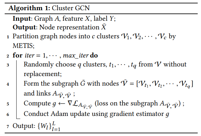
This paper doesn’t contain any theoretical proof, but reports better results than all previous work, which means it’s algorithm is intuitive but empirically efficient.

The algorithm is easy to follow according to the pseudocode below. No need for explanation.